QUESTION 14 (28 marks)
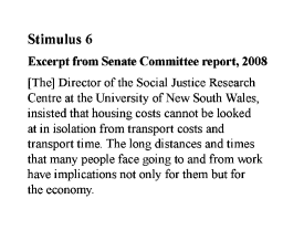
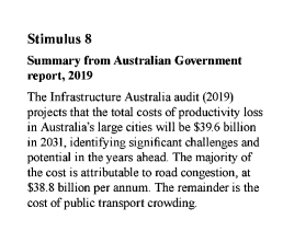
Use Stimulus 1-8 in the stimulus book to evaluate whether government intervention to influence either housing demand or housing supply would be more effective in reducing housing price pressures and improving living standards.
Stimulus book
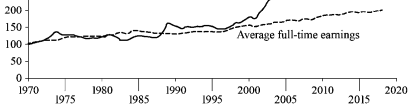
Stimulus 1
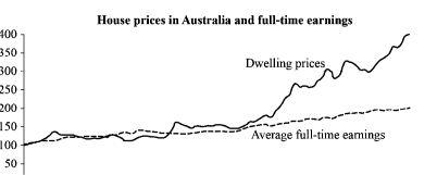
Index
Stimulus 2
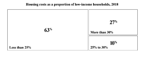
Low-income households are defined as the bottom 40% of households. Housing costs greater than 30% of household income are referred to as ‘financial housing stress’.
Stimulus 3
This stimulus has not been published for copyright reasons.
Stimulus 4
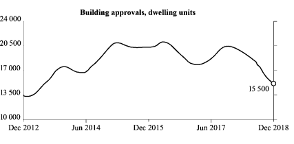
Stimulus 5
Excerpt from media release, 2019
According to a new Regional Australia Institute report, the average outer suburban Sydney worker earns $80 088, slightly more than the $71 281 pay packet of their regional city counterpart. But the cost of an average house would be halved by making a tree change!, with an outer Sydney suburban house costing $1006 105 compared to just $500 967 in regional centres.
Stimulus 7
Excerpt from media release, 2018
This stimulus has not been published for copyright reasons.
Read the media release
Property Council of Australia 2018, ‘Increasing housing supply’, 10 May, www. propertycouncil.com.au/Web/Content/ Media_Releasce/TAS/2018/Increasing_h ousing, supply.aspx 2 1 20 0 0 0 13 2160 426 3 -1 3 1 20 1 0 0 13 2160 426 3 -1 4 1 20 1 1 0 13 2160 426 3 -1 5 1 20 1 1 1 13 2160 426 3 95.000000 2 1 21 0 0 0 17 2176 8 19 -1 3 1 21 1 0 0 17 2176 8 19 -1 4 1 21 1 1 0 17 2176 8 19 -1 5 1 21 1 1 1 17 2176 8 19 96.713020 1 2 1 22 0 0 0 735 747 129 24 -1 3 1 22 1 0 0 735 747 129 24 -1 4 1 22 1 1 0 735 747 129 24 -1 5 1 22 1 1 1 735 747 52 24 96.503738 Dec 5 1 22 1 1 2 799 747 65 23 95.541367 2015 2 1 23 0 0 0 1344 293 4 440 -1 3 1 23 1 0 0 1344 293 4 440 -1 4 1 23 1 1 0 1344 293 4 440 -1 5 1 23 1 1 1 1344 293 4 440 95.000000 2 1 24 0 0 0 1010 724 400 47 -1 3 1 24 1 0 0 1010 724 400 47 -1 4 1 24 1 1 0 1072 724 2 14 -1 5 1 24 1 1 1 1072 724 2 14 77.521317 T 4 1 24 1 2 0 1010 747 400 24 -1 5 1 24 1 2 1 1010 747 47 24 94.923637 Jun 5 1 24 1 2 2 1067 747 67 23 94.923637 2017 5 1 24 1 2 3 1279 747 54 24 96.660866 Dec 5 1 24 1 2 4 1343 747 67 23 96.345566 2018 2 1 25 0 0 0 849 921 649 93 -1 3 1 25 1 0 0 849 921 649 93 -1 4 1 25 1 1 0 850 921 173 28 -1 5 1 25 1 1 1 850 921 143 28 96.704063 Stimulus 5 1 25 1 1 2 1006 922 17 26 96.721237 6 4 1 25 1 2 0 849 982 649 32 -1 5 1 25 1 2 1 849 983 112 31 96.640472 Excerpt 5 1 25 1 2 2 970 982 70 25 96.911240 from 5 1 25 1 2 3 1050 982 93 25 96.184296 Senate 5 1 25 1 2 4 1153 982 160 25 95.883179 Committee 5 1 25 1 2 5 1323 986 99 28 96.592262 report, 5 1 25 1 2 6 1431 983 67 24 96.665344 2008 2 1 26 0 0 0 848 1040 638 322 -1 3 1 26 1 0 0 848 1040 638 322 -1 4 1 26 1 1 0 850 1040 616 31 -1 5 1 26 1 1 1 850 1041 70 30 96.830734 [The] 5 1 26 1 1 2 931 1041 116 24 96.536896 Director 5 1 26 1 1 3 1057 1040 30 25 96.341934 of 5 1 26 1 1 4 1093 1040 41 25 96.601044 the 5 1 26 1 1 5 1145 1040 82 25 96.498238 Social 5 1 26 1 1 6 1239 1041 92 24 95.888214 Justice 5 1 26 1 1 7 1341 1040 125 25 96.268448 Research 4 1 26 1 2 0 849 1081 627 32 -1 5 1 26 1 2 1 849 1082 90 25 96.140656 Centre 5 1 26 1 2 2 950 1086 23 21 96.140656 at 5 1 26 1 2 3 983 1081 41 26 96.608177 the 5 1 26 1 2 4 1033 1081 144 32 96.658958 University 5 1 26 1 2 5 1188 1081 30 26 96.413055 of 5 1 26 1 2 6 1224 1083 65 24 96.936745 New 5 1 26 1 2 7 1299 1081 77 26 96.854965 South 5 1 26 1 2 8 1386 1081 90 31 96.903305 Wales, 4 1 26 1 3 0 849 1123 606 32 -1 5 1 26 1 3 1 849 1123 104 25 96.793739 insisted 5 1 26 1 3 2 963 1123 51 25 96.763519 that 5 1 26 1 3 3 1023 1123 109 32 96.763519 housing 5 1 26 1 3 4 1142 1127 67 21 96.758430 costs 5 1 26 1 3 5 1220 1127 91 21 96.789124 cannot 5 1 26 1 3 6 1320 1123 32 25 96.789124 be 5 1 26 1 3 7 1363 1123 92 25 96.065971 looked 4 1 26 1 4 0 849 1165 533 32 -1 5 1 26 1 4 1 849 1170 23 20 96.269974 at 5 1 26 1 4 2 882 1165 24 24 96.269974 in 5 1 26 1 4 3 918 1165 114 25 96.554138 isolation 5 1 26 1 4 4 1044 1165 66 25 96.645844 from 5 1 26 1 4 5 1120 1169 125 28 96.828125 transport 5 1 26 1 4 6 1256 1170 66 20 96.776276 costs 5 1 26 1 4 7 1334 1165 48 25 96.674553 and 4 1 26 1 5 0 848 1206 616 32 -1 5 1 26 1 5 1 848 1210 125 28 96.108116 transport 5 1 26 1 5 2 982 1206 67 25 96.830460 time. 5 1 26 1 5 3 1062 1206 52 25 96.764992 The 5 1 26 1 5 4 1124 1206 60 32 96.253700 long 5 1 26 1 5 5 1194 1206 126 25 96.737495 distances 5 1 26 1 5 6 1331 1206 49 25 96.777672 and 5 1 26 1 5 7 1389 1206 75 25 96.907974 times 4 1 26 1 6 0 848 1247 638 32 -1 5 1 26 1 6 1 848 1247 52 26 96.967789 that 5 1 26 1 6 2 909 1256 75 23 96.363235 many 5 1 26 1 6 3 994 1247 90 32 95.932968 people 5 1 26 1 6 4 1094 1247 57 26 95.932968 face 5 1 26 1 6 5 1160 1247 77 32 96.757370 going 5 1 26 1 6 6 1247 1252 25 21 96.593521 to 5 1 26 1 6 7 1283 1247 49 26 96.918503 and 5 1 26 1 6 8 1341 1247 68 26 96.588669 from 5 1 26 1 6 9 1418 1247 68 26 96.840820 work 4 1 26 1 7 0 848 1288 591 32 -1 5 1 26 1 7 1 848 1289 62 25 96.854561 have 5 1 26 1 7 2 921 1289 168 31 96.771378 implications 5 1 26 1 7 3 1099 1293 43 21 96.931511 not 5 1 26 1 7 4 1152 1289 59 31 96.876221 only 5 1 26 1 7 5 1222 1288 38 26 96.674721 for 5 1 26 1 7 6 1269 1289 69 25 96.350540 them 5 1 26 1 7 7 1347 1289 44 25 96.997391 but 5 1 26 1 7 8 1400 1289 39 25 96.672279 for 4 1 26 1 8 0 848 1330 178 32 -1 5 1 26 1 8 1 848 1330 41 25 96.903725 the 5 1 26 1 8 2 899 1339 127 23 95.371712 economy. 2 1 27 0 0 0 850 1541 173 28 -1 3 1 27 1 0 0 850 1541 173 28 -1 4 1 27 1 1 0 850 1541 173 28 -1 5 1 27 1 1 1 850 1541 143 28 96.247643 Stimulus 5 1 27 1 1 2 1006 1542 17 26 96.946617 8 2 1 28 0 0 0 849 1602 586 72 -1 3 1 28 1 0 0 849 1602 586 72 -1 4 1 28 1 1 0 849 1602 586 31 -1 5 1 28 1 1 1 849 1602 144 31 96.000641 Summary 5 1 28 1 1 2 1003 1602 72 25 96.000641 from 5 1 28 1 1 3 1084 1602 156 25 96.465881 Australian 5 1 28 1 1 4 1252 1602 183 25 95.854050 Government 4 1 28 1 2 0 849 1644 177 30 -1 5 1 28 1 2 1 849 1646 101 28 95.792641 report, 5 1 28 1 2 2 960 1644 66 23 96.639420 2019 2 1 29 0 0 0 848 1701 644 323 -1 3 1 29 1 0 0 848 1701 644 323 -1 4 1 29 1 1 0 848 1701 563 33 -1 5 1 29 1 1 1 848 1701 52 26 96.967804 The 5 1 29 1 1 2 910 1701 194 26 96.679161 Infrastructure 5 1 29 1 1 3 1114 1701 127 26 96.259323 Australia 5 1 29 1 1 4 1251 1701 67 26 96.259323 audit 5 1 29 1 1 5 1329 1701 82 33 96.803368 (2019) 4 1 29 1 2 0 848 1743 644 32 -1 5 1 29 1 2 1 848 1743 107 32 96.513107 projects 5 1 29 1 2 2 965 1743 51 25 96.958527 that 5 1 29 1 2 3 1026 1743 41 25 96.874908 the 5 1 29 1 2 4 1077 1743 59 25 96.871765 total 5 1 29 1 2 5 1148 1747 67 21 96.585304 costs 5 1 29 1 2 6 1226 1743 30 25 96.585304 of 5 1 29 1 2 7 1262 1743 167 32 96.575851 productivity 5 1 29 1 2 8 1441 1743 51 25 96.883537 loss 4 1 29 1 3 0 848 1784 625 32 -1 5 1 29 1 3 1 848 1784 25 25 97.003883 in 5 1 29 1 3 2 885 1784 145 25 96.362572 Australia’s 5 1 29 1 3 3 1041 1784 67 32 96.987907 large 5 1 29 1 3 4 1119 1784 70 25 96.614937 cities 5 1 29 1 3 5 1200 1784 51 25 96.875076 will 5 1 29 1 3 6 1262 1784 31 25 96.936577 be 5 1 29 1 3 7 1305 1784 69 27 96.312485 $39.6 5 1 29 1 3 8 1384 1784 89 25 96.908943 billion 4 1 29 1 4 0 849 1826 634 32 -1 5 1 29 1 4 1 849 1826 25 24 96.882332 in 5 1 29 1 4 2 885 1827 69 29 96.452660 2031, 5 1 29 1 4 3 965 1826 152 32 96.296982 identifying 5 1 29 1 4 4 1127 1826 143 31 96.508369 significant 5 1 29 1 4 5 1281 1826 142 31 96.508369 challenges 5 1 29 1 4 6 1435 1826 48 25 96.915230 and 4 1 29 1 5 0 848 1867 616 31 -1 5 1 29 1 5 1 848 1867 118 31 96.453171 potential 5 1 29 1 5 2 978 1867 25 24 96.919914 in 5 1 29 1 5 3 1014 1867 41 25 96.333458 the 5 1 29 1 5 4 1063 1875 73 23 96.921227 years 5 1 29 1 5 5 1147 1867 86 25 96.734230 ahead. 5 1 29 1 5 6 1246 1867 52 25 96.029160 The 5 1 29 1 5 7 1309 1867 114 31 96.475784 majority 5 1 29 1 5 8 1434 1867 30 25 97.016006 of 4 1 29 1 6 0 848 1908 610 32 -1 5 1 29 1 6 1 848 1908 41 26 96.987709 the 5 1 29 1 6 2 899 1913 55 21 96.857010 cost 5 1 29 1 6 3 964 1908 21 26 96.857010 is 5 1 29 1 6 4 995 1908 157 26 96.495964 attributable 5 1 29 1 6 5 1162 1913 25 21 96.801231 to 5 1 29 1 6 6 1198 1908 60 26 96.410248 road 5 1 29 1 6 7 1269 1908 154 32 96.493187 congestion, 5 1 29 1 6 8 1435 1913 23 21 96.676582 at 4 1 29 1 7 0 850 1950 632 32 -1 5 1 29 1 7 1 850 1950 70 27 96.882256 $38.8 5 1 29 1 7 2 931 1950 88 25 96.183685 billion 5 1 29 1 7 3 1029 1958 45 24 96.183685 per 5 1 29 1 7 4 1084 1958 100 17 96.576752 annum. 5 1 29 1 7 5 1197 1950 52 25 96.541542 The 5 1 29 1 7 6 1260 1950 139 25 96.332573 remainder 5 1 29 1 7 7 1409 1950 21 25 96.412239 is 5 1 29 1 7 8 1440 1950 42 25 96.812790 the 4 1 29 1 8 0 849 1992 462 32 -1 5 1 29 1 8 1 849 1996 53 21 96.988625 cost 5 1 29 1 8 2 912 1992 30 25 96.954651 of 5 1 29 1 8 3 948 1992 84 32 96.657974 public 5 1 29 1 8 4 1042 1996 126 28 96.616402 transport 5 1 29 1 8 5 1178 1992 133 32 95.014542 crowding. 2 1 30 0 0 0 56 2175 1107 27 -1 3 1 30 1 0 0 56 2175 1107 27 -1 4 1 30 1 1 0 56 2175 1107 27 -1 5 1 30 1 1 1 56 2182 29 14 96.344658 an 5 1 30 1 1 2 91 2175 124 21 95.928062 Australian 5 1 30 1 1 3 223 2175 77 27 96.582558 phrase 5 1 30 1 1 4 309 2175 124 27 96.551071 describing 5 1 30 1 1 5 442 2182 13 14 96.708923 a 5 1 30 1 1 6 463 2179 126 17 95.860451 movement 5 1 30 1 1 7 596 2175 59 21 96.777519 from 5 1 30 1 1 8 662 2175 63 21 96.833458 cities 5 1 30 1 1 9 734 2175 92 21 96.556190 towards 5 1 30 1 1 10 835 2175 97 27 96.612701 regional 5 1 30 1 1 11 941 2175 43 21 96.983002 and 5 1 30 1 1 12 993 2175 55 21 96.287025 rural 5 1 30 1 1 13 1057 2175 106 21 96.397293 locations
QCAA guide · typeset solution
QCAA sample response and mark allocation
Extended response — Question 14 (28 marks)
The response, for house prices: | M |  | M | The response: | M |
• quantifies the trend of house prices increasing (↑) over time (s1) • explains an economic relationship arising from the trend • correctly calculates a number to make meaning | 4 | • quantifies the pattern of household (HH) financial stress in low-income households (s2) • explains an economic relationship linked to the pattern | 3 | • provides a rationale for government (G) intervention to relieve house price pressures | 2 |
• quantifies the trend of house prices ↑ • explains an economic relationship arising from the trend OR • quantifies the trend of house prices ↑ • correctly calculates a number to make meaning | 3 | • quantifies the pattern of HH financial stress in low-income households OR • explains an economic relationship to low-income households | 2 | • identifies a rationale for G intervention to relieve house price pressures | 1 |
• quantifies the trend of house prices ↑ OR • identifies the trend of house prices ↑ • describes an economic relationship to house prices | 2 | • identifies that HH financial stress is linked to low-income households | 1 | • does not satisfy any of the descriptors above. | 0 |
• identifies that house prices are ↑ | 1 | • does not satisfy any of the descriptors above. | 0 | ||
• does not satisfy any of the descriptors above. | 0 | ||||
 | M |  | M |  | M |  | M | The response: | M |
• provides a detailed explanation of housing supply pressures • uses data in the explanation | 4 | • identifies that government (G) intervention in housing supply would be effective • provides a detailed explanation of how G intervention can improve housing supply • links to an economic idea | 4 | • provides a detailed explanation of housing demand pressures • uses data in the explanation | 4 | • identifies that government (G) intervention in housing demand would be effective • provides a detailed explanation of how a G intervention can shift housing demand • links to an economic idea | 4 | • draws a valid conclusion of benefits of government (G) intervention based on living standards • provides reasoning for the decision, synthesising HH demand and supply ideas • uses economic terms effectively | 3 |
• provides a detailed explanation of housing supply pressures OR • explains housing supply pressures • uses data in the explanation | 3 | • identifies that G intervention in housing supply would be effective • explains how G intervention can improve housing supply • links to an economic idea | 3 | • provides a detailed explanation of housing demand pressures OR • explains housing demand pressures • uses data in the explanation | 3 | • identifies that G intervention in housing demand would be effective • explains how a G intervention can shift housing demand • links to an economic idea | 3 | • draws a valid conclusion based on living standards • provides reasoning to support the decision | 2 |
• describes a housing supply pressure OR • identifies housing supply pressures • uses data in the identification | 2 | • identifies that G intervention can influence housing supply • identifies how G can improve housing supply | 2 | • describes a housing demand pressure OR • identifies a housing demand pressure • uses data in the identification | 2 | • identifies that G intervention can influence housing demand • identifies how a G intervention can shift housing demand | 2 | • identifies a conclusion based on living standards | 1 |
• identifies that housing supply affects housing prices | 1 | • identifies that G can influence housing supply | 1 | • identifies city and regional areas have different housing demand forces | 1 | • identifies that G can influence housing demand | 1 | • does not satisfy any of the descriptors above. | 0 |
 | M |  | M |  | M |  | M | The response: | M |
• does not satisfy any of the descriptors above. | 0 | • does not satisfy any of the descriptors above. | 0 | • does not satisfy any of the descriptors above. | 0 | • does not satisfy any of the descriptors above. | 0 | ||
QCAA sample response and marking criteria reproduced from the official guide.
Compare your working with the guide above.